This is a simple note on Turing completeness of 2-neighbourhood 1-dimensional Cellular Automata.
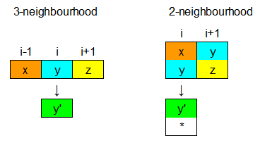
A Cellular Automaton (pl. Cellular Automata) is a model of computation based on a grid of cells that evolve according to a simple set of rules. The grid can be multi-dimensional, the most famous and studied cellular automata are 1-dimensional and 2-dimensional. Each cell can be in a particular finite state ($k$-states CA), at each step of the evolution (generation) the cell changes its state according to its current state and the state of its neighboring cells. The number of neighbours considered is finite; for a 1-dimensional CA, the usual choice is the adjacent neighbours. A m-neighbourhood 1-dimensional CA is a CA in which the next state of cell $c_i$ depends on the state of $c_i$ and the state of the $m-1$ adjacent cells; usually $c_i$ is the central cell.
Formally, if $t_n(c_i)$ is the state of cell $c_i$ at time $t_n$:
$$t_{n+1}(c_i) = f( t_n(c_{i-\ell}), …, t_n(c_{i-2}), t_n(c_{i-1}), t_n(c_i), t_n(c_{i+1}), t_n(c_{i+2}), …, t_n(c_{i+\ell}) )$$
and $m = 2\ell+1$.
For more details and basic references see: Das D. (2012) A Survey on Cellular Automata and Its Applications.
Even basic cellular automata can be Turing Complete, for example see the (controversial) proof of Turing completeness of the 3-neighbourhood Cellular Autaton identified by Rule 110 .
If only 1 neigbour is considered (i.e. the next state of a cell only depend on its current state), then we cannot achieve Turing completeness. But with 2-neighbourhood and enough states it’s possible to emulate every CA.
We give a simple proof of a simulation of a 2-states 3-neighbourhood 1-dimensional CA $A_{CA}$ by a 6-states 2-neighbourhood 1-dimensional CA $B_{CA}$. Without loss o generality we will assume that the state of cell $c_i$ at time $n+1$ depends only on the state of cell $c_i$ at time $n$ and teh state of the cell $c_{i+1}$ on its right at time $n$:
$$t_{n+1}(c_i)=f( t_n(c_i), t_n(c_{i+1}) )$$
The idea is to spend one generation to “stack” the state of the adjacent cell and then apply the original rule.
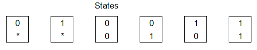
The 4 states are: $(0,*), (1,*), (0,0),(0,1),(1,0),(1,1)$
Initially, at generation 1, the cells are only in state $(0,*)$ or $(1,*)$, which represent the $0,1$ states of the original configuration of the simulated CA $A_{CA}$. We add the following rules that stack the current state of the cell $c_i$ and the current state of the adjacent cell $c_{i+1}$:
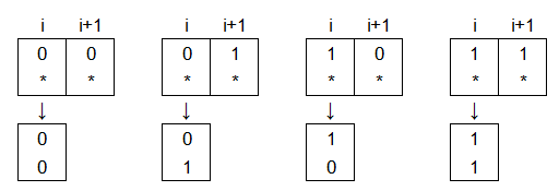
These rules are applied and lead to generation 2 of $B_{CA}$. Now every cell $c_i$ is able to “see” its current state, the current state of cell $c_{i+1}$ and the current state of cell $c_{i+2}$ and we can treat it as the original cell $c_{i+1}$ of the simulated CA and we can apply the corresponding 3-neighbourhood rule.
For every rule of the original CA $(x,y,z) \to y’$ we add the following rules:
In this way at generation 3 of $B_{CA}$, the state of cell $c_i$ is the state of generation 2 of cell $c_{i+1}$ in the simulated CA; i.e. informally the configuration is the same of the simulated CA, but shifted to the left by one cell.
The same technique can be applied to simulate more complex CAs:
Thereom 1: A $k$-states $d$-neighbourhood 1-dimensional CA can be simulated by a $k + k^{d-1}$-states 2-neighbourhood 1-dimensional CA.
Note that the simulation is only slowed by a constant factor: the $n(d-1)$-th generation of the 2-neighbourhood CA is equivalent to the $n$-th generation of the simulated $d$-neighbourhood CA. We can simulate Rule 110, so we can also conclude:
Corollary 2: There exists a 6-states 2-neighbourhood 1-dimensional CA which is (weakly) Turing Complete.
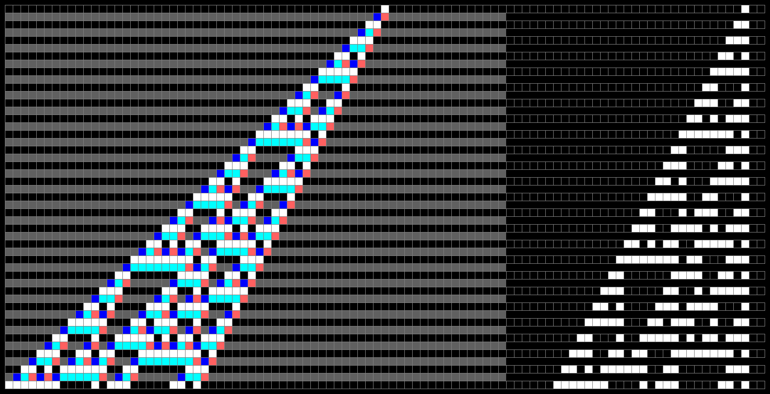
The image below represents the evolution of the 6-states 2-neighbourhood CA that simulates the Rule 110 (on the left) and the corresponding evolution of the original Rule 110 (on the right), note that odd generations are the same, but only left shifted.
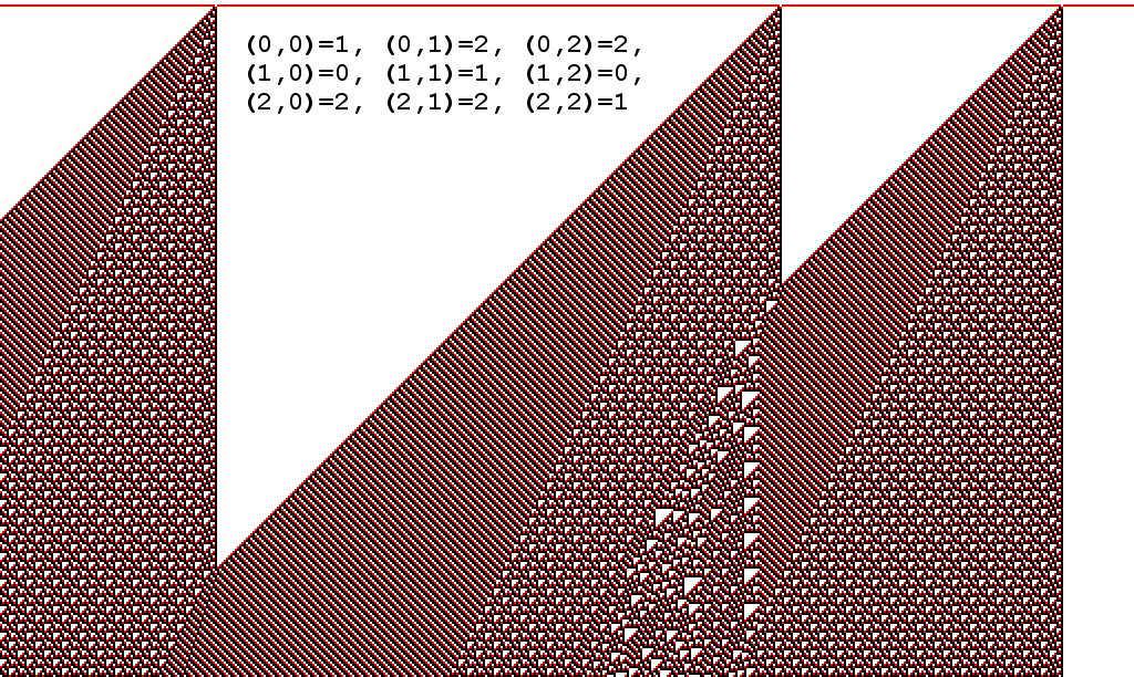
Open problem: we didn’t dig too much in the literature, but we think no one has studied the intermediate cases: $k$-states 2-neighbourhood 1D CA for $1 < k < 6$, perhaps some of them could be Turing complete. For $k=2$ (two states) the CA behaviour is simple, but for $k=3$ there are interesting examples that seem to fit in Class-4 of the classification presented in Stephen Wolfram’s A New Kind of Science, and perhaps they could be universal. For example the 3-states 2-neighbourhood CA $(1,2,2,0,1,0,2,2,1)$ exhibits the following behaviour (starting from a configuration in which all cells are 0 except three of them):